相似度计算
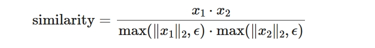
原理:余弦相似度是通过计算两个向量的夹角余弦值来衡量它们的相似度。公式为

其中 A⋅B 是向量 A 和 B 的点积

$\displaystyle \text{similarity} = \dfrac{x_1 \cdot x_2}{\max(\Vert x_1 \Vert _2, \epsilon) \cdot \max(\Vert x_2 \Vert _2, \epsilon)}$
numpy·1维
import numpy as np

# 定义两个向量
A = np.array([1, 2, 3])
B = np.array([4, 5, 6])

# 计算点积
dot_product = np.dot(A, B)

# 计算模长
norm_A = np.linalg.norm(A)
norm_B = np.linalg.norm(B)

# 计算余弦相似度
cosine_similarity = dot_product / (norm_A * norm_B)
print("余弦相似度:", cosine_similarity)
pytorch·1维
import torch

# 定义两个向量
A = torch.tensor([1.0, 2.0, 3.0])
B = torch.tensor([4.0, 5.0, 6.0])

# 计算余弦相似度
cosine_similarity = torch.cosine_similarity(A, B, dim=0)
print("余弦相似度:", cosine_similarity.item())
import torch
import torch.nn.functional as F

# 定义两个向量
A = torch.tensor([1.0, 2.0, 3.0])
B = torch.tensor([4.0, 5.0, 6.0])

# 计算余弦相似度
cosine_similarity = F.cosine_similarity(A, B, dim=0)
print("余弦相似度:", cosine_similarity.item())
pytorch·2维 import torch # 定义两个向量 A = torch.tensor([[1.0, 2.0, 3.0]]) B = torch.tensor([[1.0, 2.0, 3.0],[4.0, 5.0, 6.0]]) torch.cosine_similarity(A,B,dim=1)
tensor([1.0000, 0.9746])

如果一个矩阵只有一个元素,会进行广播
import torch

# 定义两个向量
A = torch.tensor([[1.0, 2.0, 3.0],[4.0, 5.0, 6.0]])
B = torch.tensor([[1.0, 2.0, 3.0],[4.0, 5.0, 6.0]])

torch.cosine_similarity(A,B,dim=1)
tensor([1.0000, 1.0000])

如果两个矩阵同shape,则一对一运算
|
原理:欧氏距离是衡量两个向量在空间中距离的常用方法。公式为 
numpy
import numpy as np

# 定义两个向量
A = np.array([1, 2, 3])
B = np.array([4, 5, 6])

# 计算欧氏距离
euclidean_distance = np.linalg.norm(A - B)
print("欧氏距离:", euclidean_distance)
|
原理:曼哈顿距离是计算两个向量在各维度差的绝对值之和。公式为 
numpy
import numpy as np

# 定义两个向量
A = np.array([1, 2, 3])
B = np.array([4, 5, 6])

# 计算曼哈顿距离
manhattan_distance = np.sum(np.abs(A - B))
print("曼哈顿距离:", manhattan_distance)
|
|
计算矩阵x1中每个行向量与矩阵x2中每个行向量的相似度,并提取x2中最相似行的相似度大小 numpy实现
#numpy实现

import numpy as np

# 定义两个矩阵
x1 = np.array([[1, 2, 3], [4, 5, 6]])
x2 = np.array([[7, 8, 9], [1, 2, 3]])

# 计算 x1 和 x2 的行向量的余弦相似度矩阵
def cosine_similarity_matrix(x1, x2):
    # 计算 x1 和 x2 的行向量的模
    norm_x1 = np.linalg.norm(x1, axis=1, keepdims=True)
    norm_x2 = np.linalg.norm(x2, axis=1, keepdims=True)

    # 计算 x1 和 x2 的行向量的点积
    dot_product = np.dot(x1, x2.T)

    # 计算余弦相似度矩阵
    cosine_sim_matrix = dot_product / (norm_x1 * norm_x2.T)
    return cosine_sim_matrix

cosine_sim_matrix = cosine_similarity_matrix(x1, x2)

# 提取 x1 中每个行向量与 x2 中最相似行的相似度大小
max_similarities = np.max(cosine_sim_matrix, axis=1)
print("最大相似度:", max_similarities)
x1中的每一行与x2中的每一列相乘再相加,这正是矩阵乘法的基本运算,也正好符合题目的要求
最大相似度: tensor([1.0000, 0.9982])
pytorch实现
import torch

# 定义两个矩阵
x1 = torch.tensor([[1.0, 2.0, 3.0], [4.0, 5.0, 6.0]])
x2 = torch.tensor([[7.0, 8.0, 9.0], [1.0, 2.0, 3.0]])

# 计算 x1 和 x2 的行向量的余弦相似度矩阵,x1要让行向量成为(1,n)的矩阵,于是x2为了对上x1中的元素就在0位置上新增维度
cosine_sim_matrix = torch.cosine_similarity(x1.unsqueeze(1), x2.unsqueeze(0), dim=2)

# 提取 x1 中每个行向量与 x2 中最相似行的相似度大小
max_similarities, _ = torch.max(cosine_sim_matrix, dim=1)
print("最大相似度:", max_similarities)
最大相似度: tensor([1.0000, 0.9982])
封装示例
import torch
from tpf.alg.simi import MaxSimilarity

X = torch.tensor([
    [0.3745, 0.9507, 0.7320],
    [0.5987, 0.1560, 0.1560],
    [0.0581, 0.8662, 0.6011],
    [0.7081, 0.0206, 0.9699],
    [0.8324, 0.2123, 0.1818],
    [0.1834, 0.3042, 0.5248],
    [0.4319, 0.2912, 0.6119]]).float()

x1 = X[:2,:]
x2 = X[2:,:]

model = MaxSimilarity()
sim = model(x1,x2)
sim  #tensor([0.9684, 0.9992])
数据非torch时会转为torch
import torch
import numpy as np
from tpf.alg.simi import MaxSimilarity

X = np.array([
    [0.3745, 0.9507, 0.7320],
    [0.5987, 0.1560, 0.1560],
    [0.0581, 0.8662, 0.6011],
    [0.7081, 0.0206, 0.9699],
    [0.8324, 0.2123, 0.1818],
    [0.1834, 0.3042, 0.5248],
    [0.4319, 0.2912, 0.6119]])

x1 = X[:2,:]
x2 = X[2:,:]

model = MaxSimilarity()
sim = model(x1,x2)
sim  #tensor([0.9684, 0.9992])
|
import torch
from tpf.alg.sim import TopSim

X = torch.tensor([
    [0.3745, 0.9507, 0.7320],
    [0.5987, 0.1560, 0.1560],
    [0.0581, 0.8662, 0.6011],
    [0.7081, 0.0206, 0.9699],
    [0.8324, 0.2123, 0.1818],
    [0.1834, 0.3042, 0.5248],
    [0.4319, 0.2912, 0.6119]]).float()

x1 = X[:2,:]
x2 = X[2:,:]

model = TopSim()
sim,index = model(x1,x2,n=2)
sim,index
(tensor([
    [0.9684, 0.9316],
    [0.9992, 0.7791]]),
tensor([
    [0, 3],
    [2, 4]]))
sim_data = x2[index]
sim_data[0][0]

tensor([0.0581, 0.8662, 0.6011])


#x1中索引为1的数据在x2中最相似的数据
sim_data[1][0]

tensor([0.8324, 0.2123, 0.1818])
import torch

X = torch.tensor([
    [0.3745, 0.9507, 0.7320],
    [0.5987, 0.1560, 0.1560],
    [0.0581, 0.8662, 0.6011],
    [0.7081, 0.0206, 0.9699],
    [0.8324, 0.2123, 0.1818],
    [0.1834, 0.3042, 0.5248],
    [0.4319, 0.2912, 0.6119]]).float()

x1 = X[:2,:]
x2 = X[2:,:]

# 计算余弦相似度矩阵
cosine_sim_matrix = torch.cosine_similarity(x1.unsqueeze(1), x2.unsqueeze(0), dim=2)

# 设置要获取的前n个最相似项
n = 2  # 例如获取前2个最相似的

# 获取前n个最相似的相似度值和索引
topk_similarities, topk_indices = torch.topk(cosine_sim_matrix, k=n, dim=1)

# 输出结果
print("余弦相似度矩阵:")
print(cosine_sim_matrix)
print("\n每个x1行向量与x2中前{}个最相似行向量的相似度:".format(n))
print(topk_similarities)
print("\n对应的x2中的行索引:")
print(topk_indices)
余弦相似度矩阵:
tensor([[0.9684, 0.6589, 0.5859, 0.9316, 0.8777],
        [0.3914, 0.7548, 0.9992, 0.5914, 0.7791]])

每个x1行向量与x2中前2个最相似行向量的相似度:
tensor([[0.9684, 0.9316],
        [0.9992, 0.7791]])

对应的x2中的行索引:
tensor([[0, 3],
        [2, 4]])
|
相似推荐
# 计算距离,每个样本与所有样本的距离 distance_matrix = torch.sum((x1-x2) ** 2, dim=1) index = torch.argmin(distance_matrix, dim=0) |
import numpy as np
import torch
from torch import nn

class DLCorr(nn.Module):
    def __init__(self):
        """相似推荐,从指定数据集寻找最自己最接近的数据
        - 求数据第1个元素与后面元素的相似度

        return
        -------------------------
        返回与自己最相近的数据的索引
        """
        super().__init__()

    def forward(self, X):
        """正向传播
        - 计算目标数据中与自己相似度最高的数据的索引
        """
        x1 = X[:1,:]
        x2 = X[1:,:]

        # 计算距离,每个样本与所有样本的距离
        distance_matrix = torch.sum((x1-x2) ** 2, dim=1)
        index = torch.argmin(distance_matrix, dim=0)
        return index
X = torch.tensor([
    [0.3745, 0.9507, 0.7320],
    [0.5987, 0.1560, 0.1560],
    [0.0581, 0.8662, 0.6011],
    [0.7081, 0.0206, 0.9699],
    [0.8324, 0.2123, 0.1818],
    [0.1834, 0.3042, 0.5248],
    [0.4319, 0.2912, 0.6119]]).float()

model = DLCorr()
index = model(X)
X[1:][index]
tensor([0.0581, 0.8662, 0.6011])

下面的h0要能跑通模型,大部分模型批次维度给1就行
但这个自定义模型是第1个元素与后面的元素对比,那么就至少需要2个元素
所以具体的形状还得看模型设计
#[B,C,H,W],trace需要通过实际运行一遍模型导出其静态图,故需要一个输入数据
h0 = torch.zeros(3, 3)

# trace方式,在模型设计时不要用for循环,
# 能在模型外完成的数据操作不要在模型中写,
# 不用inplace等高大上的语法,保持简单,简洁,否则onnx可能无法完全转换过去
torch.onnx.export(
    model=model,

    # model的参数,就是原来y_out = model(args)的args在这里指定了
    # 有其shape能让模型运行一次就行,不需要真实数据
    args=(h0,),

    # 储存的文件路径
    f="model_knn2.onnx",

    # 导出模型参数,默认为True
    export_params = True,

    # eval推理模式,dropout,BatchNorm等超参数固定或不生效
    training=torch.onnx.TrainingMode.EVAL,

    # 打印详细信息
    verbose=True,

    # 为输入和输出节点指定名称,方便后面查看或者操作
    input_names=["input1"],
    output_names=["output1"],

    # 这里的opset,指各类算子以何种方式导出,对应于symbolic_opset11
    opset_version=11,

    # batch维度是动态的,其他的避免动态
    dynamic_axes={
        "input1": {0: "batch"},
        "output1": {0: "batch"},
    }
)
import onnx
import onnxruntime
import numpy as np
model_onnx = onnx.load("model_knn2.onnx")  # 加载onnx模型
onnx.checker.check_model(model_onnx)  # 验证onnx模型是否加载成功

# 创建会话
session = onnxruntime.InferenceSession("model_knn2.onnx",providers=[ 'CPUExecutionProvider'])
ort_input = {session.get_inputs()[0].name: np.array(X).astype(np.float32)}  #这里要转为Numpy数组

output_name = session.get_outputs()[0].name
ort_output = session.run([output_name], ort_input)
index = ort_output[0]
X[1:][index]
tensor([0.0581, 0.8662, 0.6011])
|
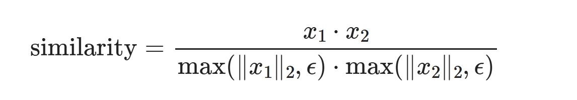
返回与第1条数据最相似数据的相似度大小及索引

$  \text{similarity} = \dfrac{x_1 \cdot x_2}{\max(\Vert x_1 \Vert _2, \epsilon) \cdot \max(\Vert x_2 \Vert _2, \epsilon)}$
import numpy as np
import torch
from torch import nn
import torch.nn.functional as F

class DLCorr(nn.Module):
    def __init__(self):
        """相似推荐,从指定数据集寻找最自己最接近的数据
        - 返回与第1条数据最相似数据的相似度大小及索引号

        return
        -------------------------
        返回与自己最相近的数据的索引
        """
        super().__init__()

    def forward(self, X):
        """正向传播
        - 计算目标数据中与自己相似度最高的数据的索引
        """
        x1 = X[:1,:]
        x2 = X[1:,:]

        # 计算余弦相似度,[0,1]越大相似度越高
        cosine_sim = F.cosine_similarity(x1, x2, dim=1)
        index = torch.argmax(cosine_sim, dim=0)
        return cosine_sim[index],index
X = torch.tensor([
    [0.3745, 0.9507, 0.7320],
    [0.5987, 0.1560, 0.1560],
    [0.0581, 0.8662, 0.6011],
    [0.7081, 0.0206, 0.9699],
    [0.8324, 0.2123, 0.1818],
    [0.1834, 0.3042, 0.5248],
    [0.4319, 0.2912, 0.6119]]).float()

model = DLCorr()
cosine_sim,index = model(X)
X[1:][index] #tensor([0.0581, 0.8662, 0.6011])
#[B,C,H,W],trace需要通过实际运行一遍模型导出其静态图,故需要一个输入数据
h0 = torch.zeros(3, 3)

# trace方式,在模型设计时不要用for循环,
# 能在模型外完成的数据操作不要在模型中写,
# 不用inplace等高大上的语法,保持简单,简洁,否则onnx可能无法完全转换过去
torch.onnx.export(
    model=model,

    # model的参数,就是原来y_out = model(args)的args在这里指定了
    # 有其shape能让模型运行一次就行,不需要真实数据
    args=(h0,),

    # 储存的文件路径
    f="model_knn2.onnx",

    # 导出模型参数,默认为True
    export_params = True,

    # eval推理模式,dropout,BatchNorm等超参数固定或不生效
    training=torch.onnx.TrainingMode.EVAL,

    # 打印详细信息
    verbose=True,

    # 为输入和输出节点指定名称,方便后面查看或者操作
    input_names=["input1"],
    output_names=["output1"],

    # 这里的opset,指各类算子以何种方式导出,对应于symbolic_opset11
    opset_version=11,

    # batch维度是动态的,其他的避免动态
    dynamic_axes={
        "input1": {0: "batch"},
        "output1": {0: "batch"},
    }
)
import onnx
import onnxruntime
import numpy as np
model_onnx = onnx.load("model_knn2.onnx")  # 加载onnx模型
onnx.checker.check_model(model_onnx)  # 验证onnx模型是否加载成功

# 创建会话
session = onnxruntime.InferenceSession("model_knn2.onnx",providers=[ 'CPUExecutionProvider'])
ort_input = {session.get_inputs()[0].name: np.array(X).astype(np.float32)}  #这里要转为Numpy数组

ort_output = session.run(None, ort_input)
cosine_sim = ort_output[0]
index = ort_output[1]
cosine_sim,X[1:][index]
(array(0.9683632, dtype=float32), tensor([0.0581, 0.8662, 0.6011])) |
|
|
|
|
多尺度+注意力
import torch
from torch import nn
from tpf.mlib.seq import SeqOne

a = torch.randn(64,512)  #模拟2维数表

model = SeqOne(seq_len=a.shape[1],  out_features=2)
model(a)[:3]
tensor([[-0.2379, -0.3309],
    [-0.6055,  0.4042],
    [ 0.2394,  0.1917]], grad_fn=SliceBackward0)
------------------------------------------------------------------------
|
from T import train
from T import X_test
from tpf.mlib.seq import SeqOne

model = SeqOne(seq_len=X_test.shape[1], out_features=2)
# model(torch.tensor(X_test).float()[:3])[:3] train(model) ------------------------------------------------------------------------ |
import numpy as np
import pandas as pd
from sklearn.datasets import load_breast_cancer
from sklearn.model_selection import train_test_split

import torch
from torch import nn

# 加载乳腺癌数据集
data = load_breast_cancer()
X = pd.DataFrame(data.data, columns=data.feature_names)
y = pd.DataFrame(data.target,columns=['target'])

X = torch.tensor(data.data).float()
y = torch.tensor(data.target).reshape(-1,1).float()

X_train, X_test, y_train,  y_test = train_test_split(X, y, test_size=0.2, random_state=42)


"""
    构建数据集
"""
import numpy as np
from torch.utils.data import Dataset
from torch.utils.data import DataLoader
import torch
from torch import nn
from torch.nn import functional as F

class MyDataSet(Dataset):

    def __init__(self,X,y):
        """
        构建数据集
        """
        self.X = X
        self.y =  y.reshape(-1)
        # self.y = y.reshape(-1,1)

    def __len__(self):
        return len(self.X)

    def __getitem__(self, idx):
        x = self.X[idx]
        y = self.y[idx]

        return torch.tensor(data=x).float(), torch.tensor(data=y).long()

train_dataset = MyDataSet(X=X_train, y=y_train)
train_dataloader = DataLoader(dataset=train_dataset, shuffle=True, batch_size=128)

test_dataset = MyDataSet(X=X_test, y=y_test)
test_dataloader = DataLoader(dataset=test_dataset, shuffle=False, batch_size=256)


# 定义训练轮次
epochs = 20
device = "cuda:0" if torch.cuda.is_available() else "cpu"


# 定义过程监控函数
def get_acc(dataloader=train_dataloader, model=None):
    accs = []
    model.to(device=device)
    model.eval()
    with torch.no_grad():
        for X,y in dataloader:
            X=X.to(device=device)
            y=y.to(device=device)
            y_pred = model(X)
            y_pred = y_pred.argmax(dim=1)
            acc = (y_pred == y).float().mean().item()
            accs.append(acc)
    return np.array(accs).mean()

# 定义训练过程
def train(model,
            epochs=epochs,
            train_dataloader=train_dataloader,
            test_dataloader=test_dataloader):
    model.to(device=device)

    # 定义优化器
    optimizer = torch.optim.SGD(params=model.parameters(), lr=1e-3)

    # 定义损失函数
    loss_fn = nn.CrossEntropyLoss()


    for epoch in range(1, epochs+1):
        print(f"正在进行第 {epoch} 轮训练:")

        model.train()
        for X,y in train_dataloader:
            X=X.to(device=device)
            y=y.to(device=device)
            # 正向传播
            y_pred = model(X)

            # 清空梯度
            optimizer.zero_grad()

            # 计算损失
            loss = loss_fn(y_pred, y)

            # 梯度下降
            loss.backward()

            # 优化一步
            optimizer.step()

        print(f"train_acc: {get_acc(dataloader=train_dataloader,model=model)}, test_acc: {get_acc(dataloader=test_dataloader,model=model)}")
|
|
简易示例 import torch from tpf.mlib.seq import SeqOne from tpf.mlib import ModelPre as mp a = torch.randn(3,512) #模拟2维数表 model = SeqOne(seq_len=a.shape[1], out_features=2) file_path = "seqone.dict" torch.save(model.state_dict(), file_path) model.load_state_dict(torch.load(file_path,weights_only=True)) 封装示例:模型保存必须以.dict后缀,否则无法使用该API import torch from tpf.mlib.seq import SeqOne from tpf.mlib import ModelPre as mp a = torch.randn(3,512) #模拟2维数表 model = SeqOne(seq_len=a.shape[1], out_features=2) file_path = "seqone.dict" y_pred = mp.predict_proba(a,model_path=file_path,model=model) y_pred array([-0.03084982, 0.01873165, -0.01635017], dtype=float32) 参数 - 数据 - 模型参数 - 模型定义 batch_size默认10W,为0表示全量预测 y_pred = mp.predict_proba(a,model_path=file_path,model=model,batch_size=1000000) y_pred array([0.03419267, 0.0257818 , 0.04169804], dtype=float32) |
|
|
SeqOne·IBM数据集
import os
import time
import numpy as np
import torch
from torch import nn
from tpf import pkl_save,pkl_load

BASE_DIR  = "/wks/datasets/ibm_aml"
file_pkl  = "ibm_aml_1.pkl"
# file_path = os.path.join(BASE_DIR, file_pkl)
file_path = file_pkl
X_train, X_test, y_train, y_test = pkl_load(file_path=file_path)
len(y_test[y_test==1]),len(y_train[y_train==1]),len(X_train)
from torch.utils.data import Dataset
from torch.utils.data import DataLoader
from tpf.dl import DataSet11
from tpf.dl import T11
from tpf.mlib.seq import SeqOne
model = SeqOne(seq_len=X_test.shape[1], out_features=2)
T11.train(model, X_train,  y_train, X_test, y_test,
        epochs=50000,
        batch_size=512,
        learning_rate=1e-4,
        model_param_path="model_params_12.pkl.dict",
        log_file="/tmp/train.log",
        per_epoch=100)
ibm_aml_1.pkl
- 去除了时间列,保留7列转化为数字
- 也就是不考虑数据之间的序列特征

SeqOne
- 提取一条数据多个特征之间的关系,也不考虑多条数据之间的关系
该模型的的精度最多达到70%

正在进行第 epoch= 1 轮训练...每轮次批次个数 =5,batch_size=512
[2025-06-21 21:04:50] train_acc: 0.697265625, test_acc: 0.68515625, good_acc:0.741796875
|
|
|
|
|
|
|
|
策略生成·决策树
|
从决策树中提取出叶子节点中数据分布集中的树分支
import numpy as np
import pandas as pd
from sklearn.datasets import load_breast_cancer
from sklearn.model_selection import train_test_split

# 加载乳腺癌数据集
data = load_breast_cancer()
X = pd.DataFrame(data.data, columns=data.feature_names)
y = pd.DataFrame(data.target,columns=['label'])
y = y['label']

from sklearn.tree import DecisionTreeClassifier
clf = DecisionTreeClassifier(
        max_depth=3,
        min_samples_leaf=30
        )
clf = clf.fit(X, y)
import matplotlib.pyplot as plt
import dtreeviz
import warnings
warnings.filterwarnings("ignore")

viz_model = dtreeviz.model(clf,
                            X_train=X,
                            y_train=y,
                            target_name='label',
                            feature_names=X.columns,
                            class_names={0:'good',1:'bad'},
                            )

v = viz_model.view(fancy=False)
v.show()
v.save("img.svg")

---------------------------------------------------------------------------
|
import numpy as np
import pandas as pd
from sklearn.datasets import load_breast_cancer
from sklearn.model_selection import train_test_split

# 加载乳腺癌数据集
data = load_breast_cancer()
X = pd.DataFrame(data.data, columns=data.feature_names)
y = pd.DataFrame(data.target,columns=['target'])
Y = y['target']

from sklearn import tree
clf = tree.DecisionTreeClassifier(
        max_depth=3,
        min_samples_leaf=50
        )
clf = clf.fit(X, Y)


import matplotlib.pyplot as plt


#设置图片的大小,想要清晰的可以设置的大点
plt.figure(figsize=(8,8),dpi=1000)

tree.plot_tree(clf)
plt.show()

# 保存矢量图格式(SVG)
plt.savefig('b.svg', format='svg', bbox_inches='tight')

|
|
|
|
|
|
|
参考
风控策略的自动化生成-利用决策树分分钟生成上千条策略