二分类混淆矩阵
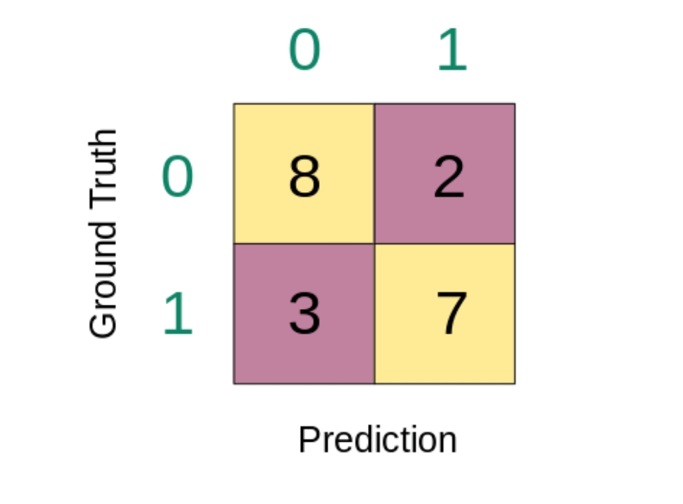
只区分 0 或 1。
它的行代表真实的类别,列代表预测的类别。
以第一行为例,真正的类别标签是 0,
有 8 个实例被预测为了 0,有 2 个实例被预测为了 1。
也就是说,在这 10 个真实标签为 0 实例中,有 8 个被正确分类,有 2 个被错误分类。
第二行这 10 个真实标签为 1 的实例中,3 个预测错了,7个预测对了。
https://cloud.tencent.com/developer/article/1935919
https://zhuanlan.zhihu.com/p/436195289
|
|
|
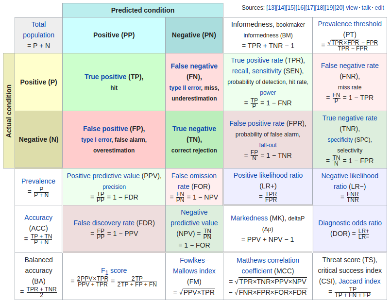
召回率(Recall):
召回率衡量了分类模型 正确预测为正例的样本数量 占 所有实际正例样本数量的比例。
计算公式为:
召回率 = TP / (TP + FN),
其中
TP表示真正例(True Positive),
FN表示假反例(False Negative)。
召回率越高,表示模型能够更好地捕捉到正例样本。
|
|
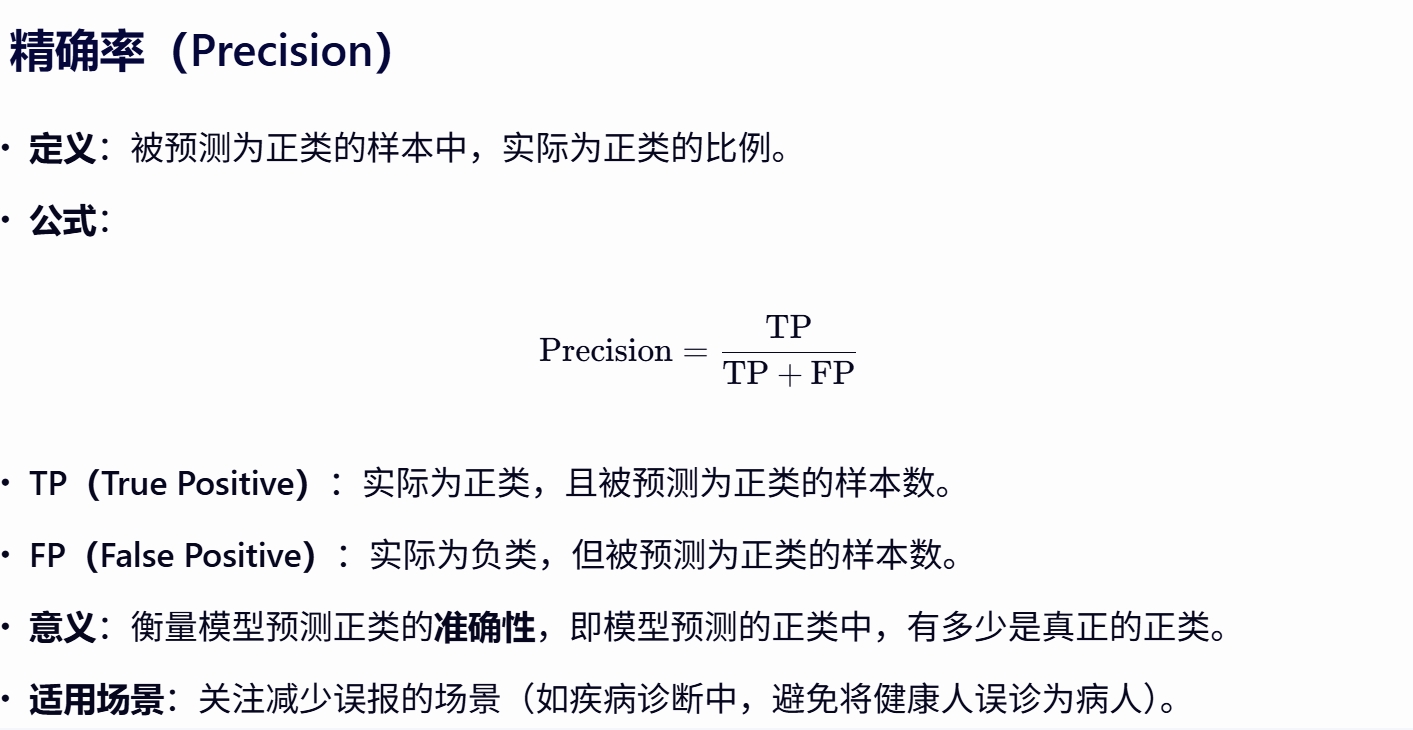
查准率(Precision):
查准率衡量了分类模型预测为正例的样本中真正为正例的比例。
计算公式为:
查准率 = TP / (TP + FP),
其中
TP表示真正例(True Positive),
FP表示假正例(False Positive)。
查准率越高,表示模型预测为正例的样本中真正为正例的比例越高。
|
|
F-度量(F-Measure):
F-度量综合考虑了召回率和查准率,是召回率和查准率的调和平均值。
计算公式为:
F-度量 = 2 * (查准率 * 召回率) / (查准率 + 召回率)。
F-度量综合了召回率和查准率的优势,能够更全面地评估分类模型的性能。
|
|
|
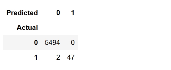
生成混淆矩阵
|
sklearn
from sklearn.metrics import confusion_matrix
# 输出混淆矩阵
print("Confusion Matrix:")
confusion_matrix(y_test, pred)
Confusion Matrix:
array([[5494, 0],
[ 2, 47]])
pandas
pd.crosstab(y_test, pred, rownames=['Actual'], colnames=['Predicted'])
|
|
```
from sklearn.metrics import confusion_matrix
y_true = ["cat", "ant", "cat", "cat", "ant", "bird"]
y_pred = ["ant", "ant", "cat", "cat", "ant", "cat"]
confusion_matrix(y_true, y_pred, labels=["ant", "bird", "cat"])
```
- labels中字符串的索引就是下面array的索引
```
array([[2, 0, 0],
[0, 0, 1],
[1, 0, 2]])
```
|
|
|
|
|
|
|
精确率
|
|
|
|
|
|
|
|
|
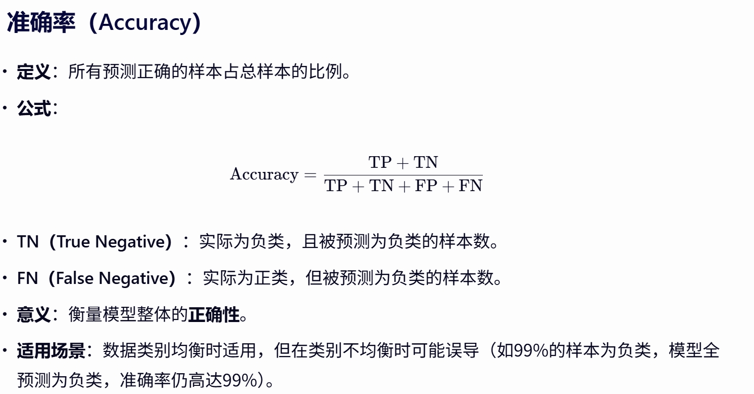
准确率
|
预测正确的数量占总数的比例
import numpy as np
np.random.seed(73)
y_pred=np.random.randint(low=0,high=2,size=(10))
y_test=np.random.randint(low=0,high=2,size=(10))
acc = (y_pred==y_test).mean()
acc = np.round(acc,decimals=4)
acc
等价于 == 转化为 true/false后的均值
---------------------------------------------------------------------
|
|
|
|
|
|
|
|
召回率

|
|
|
|
|
|
|
|
|
AUC
|
from sklearn.metrics import accuracy_score,roc_auc_score, confusion_matrix, classification_report, roc_curve, auc,f1_scor
# 预测测试集
y_pred = model.predict(X_test)
y_pred
array([1, 0, 0, 1, 1, 0, 0, 0, 1, 1, 1, 0, 1, 0, 1, 0, 1, 1, 1, 0, 1, 1,
0, 1, 1, 1, 1, 1, 1, 0, 1, 1, 1, 1, 1, 1, 0, 1, 0, 1, 1, 0, 1, 1,
1, 1, 1, 1, 1, 1, 0, 0, 1, 1, 1, 1, 1, 0, 1, 1, 1, 0, 0, 1, 1, 1,
0, 0, 1, 1, 0, 0, 1, 0, 1, 1, 1, 1, 1, 1, 0, 1, 1, 0, 0, 0, 0, 0,
1, 1, 1, 1, 1, 1, 1, 1, 0, 0, 1, 0, 0, 1, 0, 0, 1, 1, 1, 0, 1, 1,
0, 1, 0, 0])
roc_auc_score(y_test, y_pred) # 0.9464461185718965
|
|
from sklearn.metrics import accuracy_score,roc_auc_score, confusion_matrix, classification_report, roc_curve, auc,f1_score
y_scores = model.predict_proba(X_test)[:, 1] # 获取预测为恶性的概率
fpr, tpr, thresholds = roc_curve(y_test, y_scores)
roc_auc = auc(fpr, tpr)
roc_auc # 0.9977071732721913
|
|
分析差异的原因
阈值选择:
第一种方法依赖于一个固定的阈值(通常是0.5)来将概率转换为分类标签。
这个阈值可能不是最优的,导致分类性能不是最佳的。
信息利用:
第二种方法利用了完整的概率分布信息,
通过计算不同阈值下的FPR和TPR来绘制ROC曲线,并计算AUC。
这种方法通常更准确地反映了模型的性能。
哪种方法更准确?
在大多数情况下,
第二种方法(使用概率预测和 roc_curve、auc 函数)更准确地反映了模型的性能。
这是因为这种方法没有将概率预测简单地二值化为分类标签,
而是利用了模型输出的全部信息。
可能的解释
第一种方法可能由于选择了不合适的阈值(例如默认的0.5)而导致AUC值较低。
第二种方法通过考虑所有可能的阈值来全面评估模型性能,因此通常更可靠。
|
|
|
|
|
分类报告
|
```
"""
分类报告生成器 - 使用LightGBM算法和Iris数据集
"""
import numpy as np
import pandas as pd
from sklearn.datasets import load_iris
from sklearn.model_selection import train_test_split
from sklearn.metrics import classification_report, confusion_matrix, accuracy_score
from sklearn.preprocessing import StandardScaler
import lightgbm as lgb
import matplotlib.pyplot as plt
import seaborn as sns
import warnings
warnings.filterwarnings('ignore')
def load_and_prepare_data():
"""
加载和准备Iris数据集
"""
# 加载Iris数据集
iris = load_iris()
X = iris.data
y = iris.target
# 获取特征名称和目标名称
feature_names = iris.feature_names
target_names = iris.target_names
print(f"数据集形状: {X.shape}")
print(f"特征名称: {feature_names}")
print(f"目标类别: {target_names}")
print(f"类别分布: {np.bincount(y)}")
return X, y, feature_names, target_names
def train_lightgbm_model(X_train, y_train):
"""
训练LightGBM分类模型
"""
# 创建LightGBM分类器
lgb_classifier = lgb.LGBMClassifier(
objective='multiclass',
num_class=3,
metric='multi_logloss',
boosting_type='gbdt',
num_leaves=31,
learning_rate=0.05,
n_estimators=100,
random_state=42
)
# 训练模型
print("\n训练LightGBM模型...")
lgb_classifier.fit(X_train, y_train)
return lgb_classifier
from tpf.mlib import ModelEval as me
def main():
"""
主函数:执行完整的分类报告生成流程
"""
print("LightGBM分类报告生成器 - Iris数据集")
print("=" * 50)
# 1. 加载和准备数据
X, y, feature_names, target_names = load_and_prepare_data()
# 2. 划分训练集和测试集
X_train, X_test, y_train, y_test = train_test_split(
X, y, test_size=0.3, random_state=42, stratify=y
)
print(f"\n数据集划分:")
print(f"训练集大小: {X_train.shape[0]}")
print(f"测试集大小: {X_test.shape[0]}")
# 3. 特征标准化
scaler = StandardScaler()
X_train_scaled = scaler.fit_transform(X_train)
X_test_scaled = scaler.transform(X_test)
# 4. 训练LightGBM模型
model = train_lightgbm_model(X_train_scaled, y_train)
# 生成CSV格式的分类报告
# cls_report(report, target_names)
y_pred = model.predict(X_test_scaled)
me.cls_report(y_label=y_test,y_pred=y_pred, label_names=target_names, output_path="/tmp/a.csv")
# 10. 生成CSV格式的混淆矩阵
# cls_mat(cm, target_names)
me.cls_mat(y_label=y_test, y_pred=y_pred, label_names=target_names, output_path="/tmp/b.csv")
print("\n分类报告生成完成!")
print("=" * 50)
if __name__ == "__main__":
main()
```
|
|
混淆矩阵 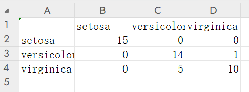
分类报告 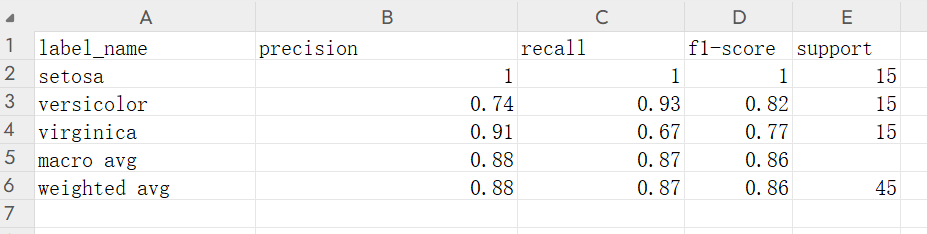
|
|
支持字符比较 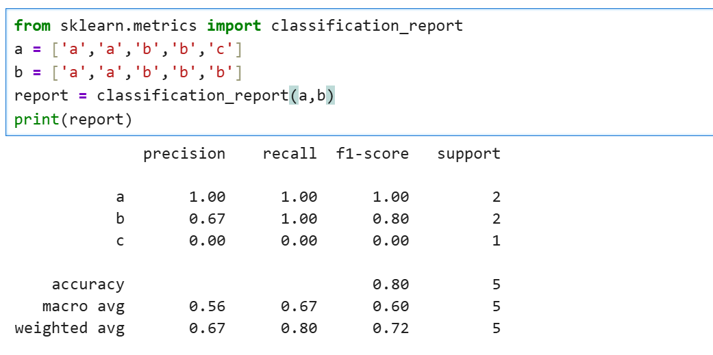
支持返回字典
```
from sklearn.metrics import classification_report
a = ['a','a','b','b','c']
b = ['a','a','b','b','b']
report = classification_report(a,b,output_dict=True)
report
```
```
{'a': {'precision': 1.0, 'recall': 1.0, 'f1-score': 1.0, 'support': 2.0},
'b': {'precision': 0.6666666666666666,
'recall': 1.0,
'f1-score': 0.8,
'support': 2.0},
'c': {'precision': 0.0, 'recall': 0.0, 'f1-score': 0.0, 'support': 1.0},
'accuracy': 0.8,
'macro avg': {'precision': 0.5555555555555555,
'recall': 0.6666666666666666,
'f1-score': 0.6,
'support': 5.0},
'weighted avg': {'precision': 0.6666666666666666,
'recall': 0.8,
'f1-score': 0.72,
'support': 5.0}}
```
|
|
|
|
|
综合计算
|
精确率
准确率
召回率
auc
F1 值
|
|
|
|
|
|
|
|
|